Learn a Reward Function using Maximum Conditional Entropy Inverse Reinforcement Learning#
Here, we’re going to take a tabular environment with a pre-defined reward function, Cliffworld, and solve for the optimal policy. We then generate demonstrations from this policy, and use them to learn an approximation to the true reward function with MCE IRL. Finally, we directly compare the learned reward to the ground-truth reward (which we have access to in this example).
Cliffworld is a POMDP, and its “observations” consist of the (partial) observations proper and the (full) hidden environment state. We use DictExtractWrapper to extract only the hidden states from the environment, turning it into a fully observable MDP to make computing the optimal policy easy.
from functools import partial

from seals import base_envs
from seals.diagnostics.cliff_world import CliffWorldEnv
from stable_baselines3.common.vec_env import DummyVecEnv

import numpy as np

from imitation.algorithms.mce_irl import (
    MCEIRL,
    mce_occupancy_measures,
    mce_partition_fh,
    TabularPolicy,
)
from imitation.data import rollout
from imitation.rewards import reward_nets

env_creator = partial(CliffWorldEnv, height=4, horizon=40, width=7, use_xy_obs=True)
env_single = env_creator()

state_env_creator = lambda: base_envs.ExposePOMDPStateWrapper(env_creator())

# This is just a vectorized environment because `generate_trajectories` expects one
state_venv = DummyVecEnv([state_env_creator] * 4)
Then we derive an expert policy using Bellman backups. We analytically compute the occupancy measures, and also sample some expert trajectories.
_, _, pi = mce_partition_fh(env_single)

_, om = mce_occupancy_measures(env_single, pi=pi)

rng = np.random.default_rng()
expert = TabularPolicy(
    state_space=env_single.state_space,
    action_space=env_single.action_space,
    pi=pi,
    rng=rng,
)

expert_trajs = rollout.generate_trajectories(
    policy=expert,
    venv=state_venv,
    sample_until=rollout.make_min_timesteps(5000),
    rng=rng,
)

print("Expert stats: ", rollout.rollout_stats(expert_trajs))
Expert stats: {'n_traj': 128, 'return_min': 296.0, 'return_mean': 325.109375, 'return_std': 9.347655433817348, 'return_max': 334.0, 'len_min': 40, 'len_mean': 40.0, 'len_std': 0.0, 'len_max': 40}
Training the reward function#
The true reward here is not linear in the reduced feature space (i.e \((x,y)\) coordinates). Finding an appropriate linear reward is impossible, but an MLP should Just Work™.
import matplotlib.pyplot as plt
import torch as th


def train_mce_irl(demos, hidden_sizes, lr=0.01, **kwargs):
    reward_net = reward_nets.BasicRewardNet(
        env_single.observation_space,
        env_single.action_space,
        hid_sizes=hidden_sizes,
        use_action=False,
        use_done=False,
        use_next_state=False,
    )

    mce_irl = MCEIRL(
        demos,
        env_single,
        reward_net,
        log_interval=250,
        optimizer_kwargs=dict(lr=lr),
        rng=rng,
    )
    occ_measure = mce_irl.train(**kwargs)

    imitation_trajs = rollout.generate_trajectories(
        policy=mce_irl.policy,
        venv=state_venv,
        sample_until=rollout.make_min_timesteps(5000),
        rng=rng,
    )
    print("Imitation stats: ", rollout.rollout_stats(imitation_trajs))

    plt.figure(figsize=(10, 5))
    plt.subplot(1, 2, 1)
    env_single.draw_value_vec(occ_measure)
    plt.title("Occupancy for learned reward")
    plt.xlabel("Gridworld x-coordinate")
    plt.ylabel("Gridworld y-coordinate")
    plt.subplot(1, 2, 2)
    _, true_occ_measure = mce_occupancy_measures(env_single)
    env_single.draw_value_vec(true_occ_measure)
    plt.title("Occupancy for true reward")
    plt.xlabel("Gridworld x-coordinate")
    plt.ylabel("Gridworld y-coordinate")
    plt.show()

    plt.figure(figsize=(10, 5))
    plt.subplot(1, 2, 1)
    env_single.draw_value_vec(
        reward_net(th.as_tensor(env_single.observation_matrix), None, None, None)
        .detach()
        .numpy()
    )
    plt.title("Learned reward")
    plt.xlabel("Gridworld x-coordinate")
    plt.ylabel("Gridworld y-coordinate")
    plt.subplot(1, 2, 2)
    env_single.draw_value_vec(env_single.reward_matrix)
    plt.title("True reward")
    plt.xlabel("Gridworld x-coordinate")
    plt.ylabel("Gridworld y-coordinate")
    plt.show()

    return mce_irl
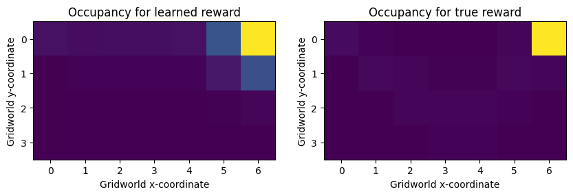
As you can see, a linear reward model cannot fit the data. Even though we’re training the model on analytically computed occupancy measures for the optimal policy, the resulting reward and occupancy frequencies diverge sharply.
train_mce_irl(om, hidden_sizes=[])
--------------------------
| grad_norm   | 19.9     |
| iteration   | 0        |
| linf_delta  | 31.1     |
| weight_norm | 0.883    |
--------------------------
--------------------------
| grad_norm   | 3.27     |
| iteration   | 250      |
| linf_delta  | 17.9     |
| weight_norm | 2.56     |
--------------------------
--------------------------
| grad_norm   | 1.95     |
| iteration   | 500      |
| linf_delta  | 14.7     |
| weight_norm | 4.14     |
--------------------------
--------------------------
| grad_norm   | 1.42     |
| iteration   | 750      |
| linf_delta  | 12.9     |
| weight_norm | 5.59     |
--------------------------
Imitation stats:  {'n_traj': 128, 'return_min': -12.0, 'return_mean': 115.9375, 'return_std': 40.625336537067604, 'return_max': 225.0, 'len_min': 40, 'len_mean': 40.0, 'len_std': 0.0, 'len_max': 40}

<imitation.algorithms.mce_irl.MCEIRL at 0x7f0d18132c10>
Now, let’s try using a very simple nonlinear reward model: an MLP with a single hidden layer. We first train it on the analytically computed occupancy measures. This should give a very precise result.
train_mce_irl(om, hidden_sizes=[256])
--------------------------
| grad_norm   | 72.7     |
| iteration   | 0        |
| linf_delta  | 30.8     |
| weight_norm | 11.4     |
--------------------------
--------------------------
| grad_norm   | 0.256    |
| iteration   | 250      |
| linf_delta  | 0.202    |
| weight_norm | 17.5     |
--------------------------
--------------------------
| grad_norm   | 0.28     |
| iteration   | 500      |
| linf_delta  | 0.128    |
| weight_norm | 19.7     |
--------------------------
--------------------------
| grad_norm   | 0.19     |
| iteration   | 750      |
| linf_delta  | 0.0468   |
| weight_norm | 22       |
--------------------------
Imitation stats:  {'n_traj': 128, 'return_min': 289.0, 'return_mean': 324.7890625, 'return_std': 9.140100812961187, 'return_max': 334.0, 'len_min': 40, 'len_mean': 40.0, 'len_std': 0.0, 'len_max': 40}

<imitation.algorithms.mce_irl.MCEIRL at 0x7f0d18132d30>
Then we train it on trajectories sampled from the expert. This gives a stochastic approximation to occupancy measure, so performance is a little worse. Using more expert trajectories should improve performance – try it!
mce_irl_from_trajs = train_mce_irl(expert_trajs[0:10], hidden_sizes=[256])
--------------------------
| grad_norm   | 135      |
| iteration   | 0        |
| linf_delta  | 33.7     |
| weight_norm | 11.4     |
--------------------------
--------------------------
| grad_norm   | 2.21     |
| iteration   | 250      |
| linf_delta  | 0.518    |
| weight_norm | 20.4     |
--------------------------
--------------------------
| grad_norm   | 5.83     |
| iteration   | 500      |
| linf_delta  | 0.511    |
| weight_norm | 34.8     |
--------------------------
--------------------------
| grad_norm   | 10.7     |
| iteration   | 750      |
| linf_delta  | 0.512    |
| weight_norm | 51.4     |
--------------------------
Imitation stats:  {'n_traj': 128, 'return_min': 296.0, 'return_mean': 325.7265625, 'return_std': 7.710296325926374, 'return_max': 334.0, 'len_min': 40, 'len_mean': 40.0, 'len_std': 0.0, 'len_max': 40}
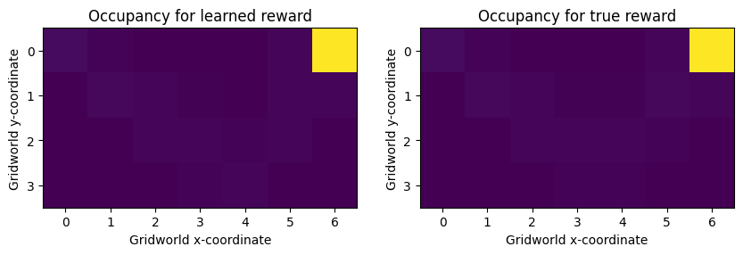

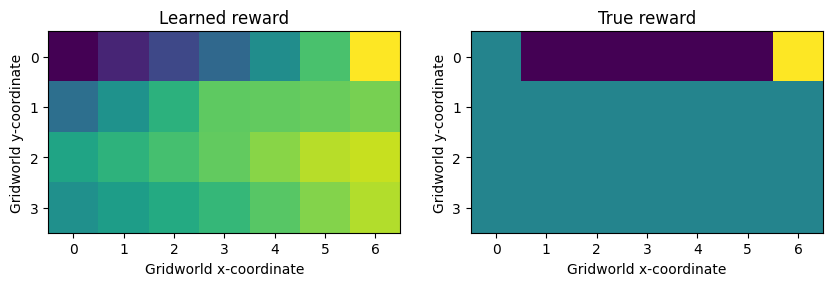
While the learned reward function is quite different from the true reward function, it induces a virtually identical occupancy measure over the states. In particular, states below the top row get almost the same reward as top-row states. This is because in Cliff World, there is an upward-blowing wind which will push the agent toward the top row with probability 0.3 at every timestep.
Even though the agent only gets reward in the top row squares, and maximum reward in the top righthand square, the reward model considers it to be almost as good to end up in one of the squares below the top rightmost square, since the wind will eventually blow the agent to the goal square.